GPhys では多次元で線形補間できます.補間メソッドは interpolate という名前で,コアの部分はCによる拡張ライブラリとして実装されています. このメソッドの上に,マウスでの切り出しや格子点あわせのメソッドが提供されてます.
本稿の対応バージョン: GPhys 1.0.0以降
準備: NCEP 再解析の気温データ air.2010JanFeb.nc *1 を適当な作業ディレクトリにダウンロードし,そこに cd します.
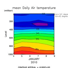
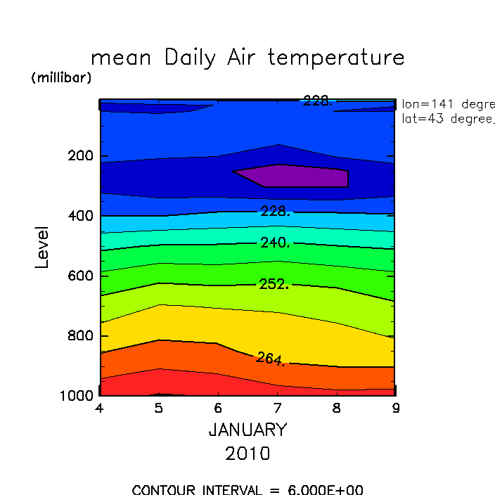
補間に使う GPhys のメソッドは interpolate です.札幌(141E,43N)の気温の高度時間断面を補間で求めて図示してみましょう.
サンプルプログラム interpo1_sapporo.rb:
require "numru/ggraph"
include NumRu

#< open data / select a date for conciseness >

temp = GPhys::IO.open("air.2010JanFeb.nc","air").cut(
          "time"=>Date.parse("2010-01-04")..Date.parse("2010-01-9"))

#< prepare new coordinates and interpolate >

lon = VArray.new(NArray[141.0],{"units"=>"degree_east"},"lon")
lat = VArray.new(NArray[43.0],{"units"=>"degree_north"},"lat")
tsapporo = temp.interpolate(lon,lat)[0,0,false]

#< graphics >

iws = (ARGV[0] || 1).to_i
DCL.swpset('ldump',true) if iws==4
DCL.swpset('iwidth',700)
DCL.swpset('iheight',700)
DCL.sgpset('isub', 96)      # control character of subscription: '_' --> '`'
DCL.glpset('lmiss',true)
DCL.gropn(iws)
GGraph::tone_and_contour tsapporo, true, "exchange"=>true
DCL.grcls
実行
ruby interpo1_sapporo.rb
実行結果(full size) :
interpolate メソッドでは,補間後の座標を引数として与えます.ここでは,
"lon", "lat" がそれです.それぞれ長さ1の座標軸 (VArrayクラス) になってますので,
緯度経度の一点を指定することになります.長さ 1 でも,次元として残り4次元のままですので,
interpolate 直後に [0,0,false] を適用して(0でその次元の最初の要素を指定して)2次元化しています.
なお,interpolate は座標軸の名前で対応を判断しますので,次元 ("lon", "lat") の名付けは必須です.
一方,単位 ("degree_east" 等) は食い違えば無視されるので,
与えなくても構いません(警告は表示されます).ただし,"km" と "m" や "days since 2010-01-01"
と "hours since 1900-01-01" のように換算可能な単位については換算します.
なお,一点を指定する場合,名前と値の組を Hash で指定することもできます. ただし,GPhys 1.0.0 では,Hash で対応する他のケースとの分離が不十分 であるという事情があり,必ずしも使いやすくないかもしれません. 次のリリースでは
tsapporo = temp.interpolate({"lon"=>141.0, "lat"=>43.0})
とできるようにする予定ですが,現状では, interpo1_sapporo__.rb のようにする必要があります.
もしも補間先として領域外を指定すれば,線形外挿になります.ごく近傍以外への外挿は一般に好ましくないので注意してください.
なお,interpolate でなく,cut メソッドを使って,
tnearS = temp.cut({"lon"=>141.0, "lat"=>43.0})
とすると,141E, 43N にもっとも近い経度,緯度の格子点を選ぶことになります. この場合,演算は必要ありませんので,tnearS の実体は temp のサブセットへのマッピングとなります. (以上において { } は省略できます.)
もちろん補間先の座標は複数点にできます.例えば lon, lat を 5 点ずつとる場合, 5×5の格子点(全25点)に内挿したい場合と,緯度経度の任意の組み合わせで計5点に内挿したい場合があるでしょう.interpolate では,前者は
temp.interpolate(lon,lat)
後者は
temp.interpolate([lon,lat])
という形で実現できます(ここで,lon, lat は5点の格子点を表す
VArray).
つまり,[lon,lat] のように配列にまとめて引数とすると,
[ [lon[0],lat[0]], [lon[1],lat[1]],..]
という形の組み合わせで内挿先の格子点をとります.以下に,実際に動作するサンプルプログラムを示します.
サンプルプログラム interpo2_grid_slice.rb:
require "numru/ggraph"
include NumRu

#< open data / select a date for conciseness >

temp = GPhys::IO.open("air.2010JanFeb.nc","air")[false,3..8]  # 3..8 => Jan 4-9

#< prepare new coordinates and interpolate >

lon = VArray.new( NArray.float(5).indgen!+135, {"units"=>"degree_east"},"lon")
lat = VArray.new( NArray.float(5).indgen!+34, {"units"=>"degree_north"},"lat")
t_grid = temp.interpolate(lon,lat)
t_slice = temp.interpolate([lon,lat])

#< print >
p "t_grid", t_grid
p "t_slice", t_slice

#< graphics >

iws = (ARGV[0] || 1).to_i
DCL.swpset('ldump',true) if iws==4
DCL.swpset('iwidth',800)
DCL.swpset('iheight',400)
DCL.sgpset('isub', 96)      # control character of subscription: '_' --> '`'
DCL.glpset('lmiss',true)
DCL.gropn(iws)
DCL.sldiv('y',2,1)
GGraph.set_fig "itr"=>10
GGraph.set_map "coast_japan"=>true
GGraph.tone_and_contour t_grid
GGraph.set_fig "itr"=>1
GGraph.tone_and_contour t_slice.cut('level'=>850)
DCL.grcls
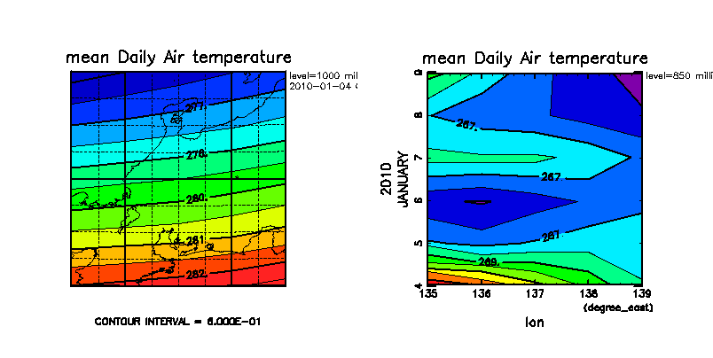
実行結果を下に示します.図だと2番目のは経度についてしか示されないので 緯度も変化しながら内挿してることが分かりにくいです(この点の改善は GGraph の将来課題),標準出力を見ると,lon という軸に lat という軸が関係づけられていることがわかります(AssocCoordsの欄).
実行結果
実行と標準出力:
% ruby interpo2_grid_slice.rb 4
"t_grid"
<GPhys grid=<4D grid <axis pos=<'lon' float[5] val=[135.0,136.0,137.0,138.0,...]>>
        <axis pos=<'lat' float[5] val=[34.0,35.0,36.0,37.0,...]>>
        <axis pos=<'level' shape=[17]  subset of a NumRu::VArrayNetCDF>>
        <axis pos=<'time' shape=[6]  subset of a NumRu::VArrayNetCDF>>>
   data=<'air' sfloat[5, 5, 17, 6] val=[282.029998779297,282.181213378906,282.332397460938,282.561614990234,...]>>
"t_slice"
<GPhys grid=<3D grid <axis pos=<'lon' float[5] val=[135.0,136.0,137.0,138.0,...]>>
        <axis pos=<'level' shape=[17]  subset of a NumRu::VArrayNetCDF>>
        <axis pos=<'time' shape=[6]  subset of a NumRu::VArrayNetCDF>>
        <AssocCoords  <'lat' float[5] val=[34.0,35.0,36.0,37.0,...]>
                {["lon"]=>["lat"]}>>
   data=<'air' sfloat[5, 17, 6] val=[282.029998779297,280.350006103516,279.000396728516,277.755218505859,...]>>
 *** MESSAGE (SWDOPN) ***  GRPH1 : STARTED / IWS =  4.
 *** WARNING (STSWTR) ***  WORKSTATION VIEWPORT WAS MODIFIED.
 *** MESSAGE (SWPCLS) ***  GRPH1 : PAGE =   1 COMPLETED.
 *** MESSAGE (SWDCLS) ***  GRPH1 : TERMINATED.
準備: NCEP 再解析の気温データ air.2010JanFeb.nc *2 を適当な作業ディレクトリにダウンロードし,そこに cd します.また,irb用共通スタートアップファイル irbrc_ggraph.rb をホームディレクトリ "~" または現在のディレクトリにダウンロードします.以下ではホームディレクトリに置いたものとして話を進めます.
これまでの例では,補間先の座標はあらかじめプログラム中で与えました.
interpolate の応用メソッドである mouse_cut を使うと,
マウスで指定することができます.2次元で図示して対話的に断面を切り出すのです.
ここでは,試行錯誤で繰り返すのに適する irb で実行してみましょう(後に実行プログラムも掲載します).まず,コマンドラインに次を入力します (irbrc_ggraph.rbファイルをカレントディレクとにおいた場合は,"~/" の部分はとって入力).
irb -r ~/irbrc_ggraph.rb
すると,irb の入力プロンプトが現れるので,以下をコピー&ペーストで流し込みます.
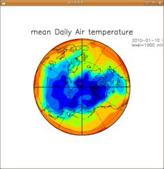
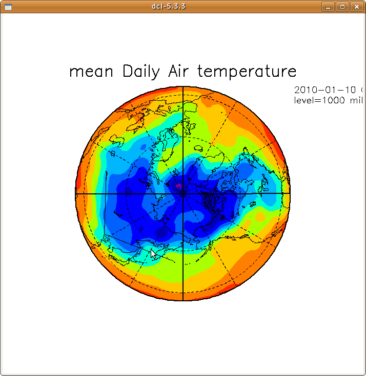
temp = gpopen("air.2010JanFeb.nc/air").cut("time"=>Date.parse("2010-01-10"))
set_map "coast_world"=>true
set_fig "itr"=>30
tone temp
tcut,line = temp.mouse_cut(0,1)
next_fig "itr"=>2 ; tone tcut; color_bar
5行目の,temp.mouse_cut(0,1) を実行すると,
'*** Waiting for mouse click. Click 2 points in the current viewport.
という表示がでて,マウスクリックを待ちますので,描画されてる範囲内で2点クリックしてください. 範囲外をクリックすると,やりなおしが求められます.
mouse_cut の引数 (0,1) で指定しているのは,図のx,y軸に相当する次元が temp においては何番目の次元化ということです(0から数えます."lon", "lat" のように名前でも指定できます). クリックする図は mouse_cut 呼び出しよりも前に書いたものなので,図の軸が切り出し対象のどの軸に当たるかを指定する必要があるのです.
mouse_cut の戻り値は2つあり,最初の (tcut) は切り出しで得られた GPhys オブジェクト,2番めの (line) は,切り出しにつかった線分 (DCLMouseLineクラスのオブジェクト) です. なお,mouse_cut を呼ぶ前の図では カラーバーを表示しないでください. 表示すると,DCL のビューポートの取り直しが発生するため,正しく断面がとれません. (この問題は将来の版で解決するかもしれません.)
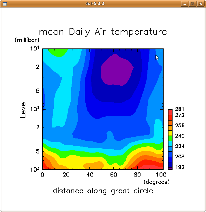
さて,2点をクリックすると,その間を結ぶ線分が表示され(下の図a: わかりにくいですが,日本から北極を通って反対側に伸びる線),その線に沿って断面を切り出し,次の行で図示されます(図b). その間に何点とるかは2点間の格子点数に応じておよその分解能を保存するよう決められます. なお,図のように,地図投影している場合も,図の直線にそって切り出されます.
地図投影の場合,主座標軸は大円上の距離(単位は度)になります. それが最良とは限りませんが,投影された線分上の距離にすると単位が不明確ですので. 切り出し結果 tcut を p コマンドで表示すると,緯度経度が補助座標として入っていることがわかります:
irb(main)> p tcut
<GPhys grid=<2D grid <axis pos=<'dist' float[69] val=[0.0,0.28327150864204,0.566310823555379,0.849106337409739,...]>>
        <axis pos=<'level' shape=[17]  subset of a NumRu::VArrayNetCDF>>
        <AssocCoords  <'lon' float[69] val=[20.2975883483887,20.4134693145752,20.5362205505371,20.6664447784424,...]>
                <'lat' float[69] val=[79.9568328857422,80.2394027709961,80.5216979980469,80.8037033081055,...]>
                {["dist"]=>["lon", "lat"]}>>
   data=<'air' sfloat[69, 17] val=[250.371932983398,248.930969238281,247.500518798828,246.070541381836,...]>>
描画が地図投影でない場合,2つの座標軸のうち,クリックでとった幅が広い方が主座標変数,もう一方が補助座標変数となります.
以上,irb を使う例を示しましたが,同じことがプログラム interpo3_mouse.rb でも実行できます.
さて,一度マウスで行った切り出しは,繰り替えして行うことができます.たとえば,(("uwnd")) という変数に風速が入っていたとすると,
ucut,line = unwd.mouse_cut_repeat
で直前の切り出しを繰り返します(直前に使った補間先の座標変数が保存されているのでそれを使う).
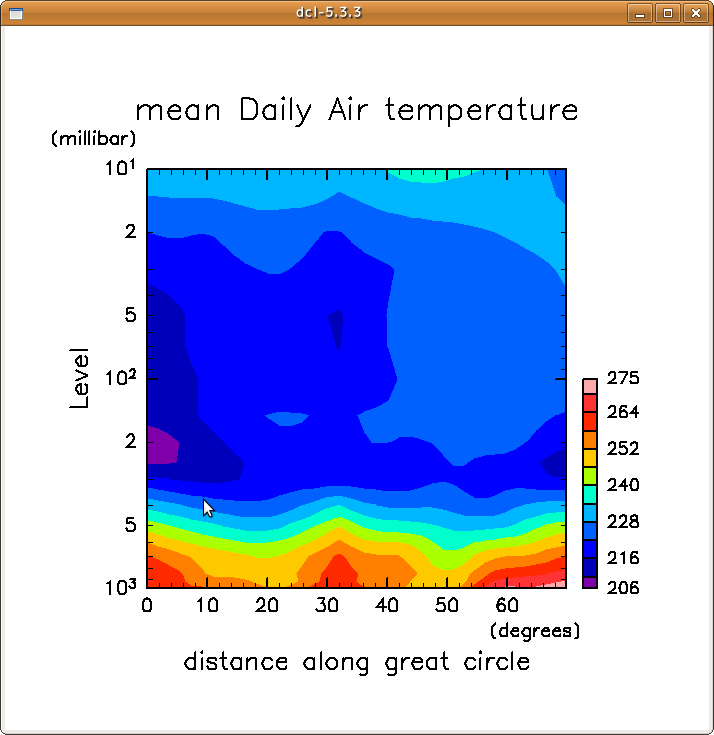
切り出しは2点間だけでなく3点以上の折れ線にそってもできます:
tone temp
tcut,line = temp.mouse_cut(0,1,3)
next_fig "itr"=>2 ; tone tcut; color_bar
mouse_cut の第3引数では,(折れ)線の点数を指定します. 省略値は2となっていますので,デフォルトは2点間の線分上での切り出しなのです. 下の図は,東アジアで3点とった例を示します.
準備: NCEP 再解析の気温 air.2010JanFeb.nc および東西風 uwnd.2010JanFeb.nc の日平均値データ *3 を適当な作業ディレクトリにダウンロードし,そこに cd します.
大気・海洋の数値モデリングでは通常,凹凸のある地表面が一定値となるような鉛直座標(σ座標など)が用いられます.これを,高度や気圧に基づいた座標に変換するのは基本的な作業です.また,温位のように比較的単調性・保存性の高い物理量を座標軸にとることも行われます.このような変換では,変換対象は1次元(以上の例では鉛直座標)ですが,変換前後の座標の対応は他の空間軸や時間軸の関数となります.ここではそのような変換を扱います.
GPhys オブジェクトは,配列の各軸に対応する1次元の(主)座標変数に加え,1〜複数の軸に対応できる1〜多次元の「補助座標」を持つことができます.interpolate メソッドの引数にできるのは,主座標になりうる1次元の VArray のみですが,それぞれの VArray は多次元の補助座標に対応できます(対応は名前で決まりますので,ある補助座標に対応する1次元 VArray とは,その補助座標と同じ同じ名前をもつ VArray です).標記の座標変換は,補助座標を使って実現します.
ここでは,温位座標に変換するサンプルプログラムを使って説明します.
サンプルプログラム interpo4_theta_coord.rb:
require "numru/ggraph"
include NumRu

#< interpret command-line arguments >

iws = (ARGV[0] || 1).to_i

#< open data >

temp = GPhys::IO.open("air.2010JanFeb.nc","air")[false,2..-1,{0..20,10}]
uwnd = GPhys::IO.open("uwnd.2010JanFeb.nc","uwnd")[false,2..-1,{0..20,10}]

#< calculate potential temperature (theta) >

prs = temp.axis("level").to_gphys
p00 =  UNumeric[1000.0, "millibar"]
kappa = 2.0 / 7.0
pfact = (prs/p00)**(-kappa)
theta = temp * pfact
theta.name = "theta"
theta.long_name = "potential temperature"

#< set theta as an associated coordinate >

uwnd.set_assoc_coords([theta])
p "uwnd:", uwnd

#< prepare a theta coordinate variable >

tht_crd = VArray.new( NArray[300.0,350.0, 400.0, 500.0, 700.0, 800.0],
                      {"units"=>"K"}, "theta")

#< transform the vertical coordinate to theta >

uwnd_ontht = uwnd.interpolate("level"=>tht_crd)

#< graphics >

DCL.swpset('iwidth',800)
DCL.swpset('iheight',400)
DCL.swpset('ldump',true) if iws==4
DCL.gropn(iws)
DCL.sldiv('y',2,1)
DCL.sgpset('isub', 96)      # control character of subscription: '_' --> '`'
DCL.glpset('lmiss',true)

GGraph::set_fig "itr"=>2,"viewport"=>[0.16,0.73,0.2,0.8]
GGraph::tone_and_contour uwnd.mean(0),true
GGraph::color_bar

GGraph::set_fig "itr"=>1
GGraph::tone_and_contour uwnd_ontht.mean(0),true
GGraph::color_bar

DCL.grcls
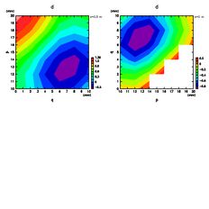
実行
ruby interpo4_theta_coord.rb
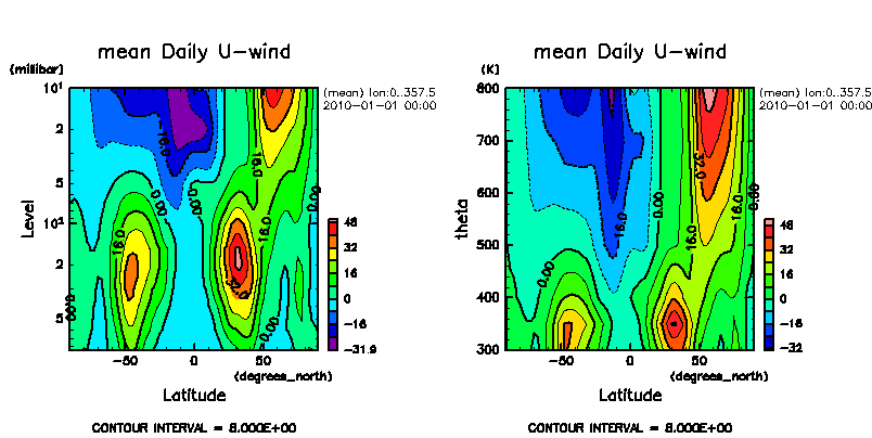
実行結果(full size)
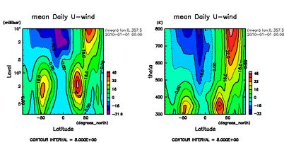
プログラムは少々長いですが,多くは準備や描画部分であり,座標変換そのものに関する部分は短くなっています. ファイルを開いたあと,θ = T*(p00/p)^κ (pは気圧,p00 は定数=1000hPa, κ = 2/7) によって,温位θを求めます.θは鉛直にほぼ単調増大となります.
ついで,
uwnd.set_assoc_coords([theta])
によって,theta を uwnd の補助座標とします. set_assoc_coords の引数は,補助座標にする GPhys オブジェクトを並べた配列になります *4. この時点で uwnd を p で表示すると,次のようになります.
"uwnd:"
<GPhys grid=<4D grid <axis pos=<'lon' shape=[144]  subset of a NumRu::VArrayNetCDF>>
        <axis pos=<'lat' shape=[73]  subset of a NumRu::VArrayNetCDF>>
        <axis pos=<'level' shape=[15]  subset of a NumRu::VArrayNetCDF>>
        <axis pos=<'time' shape=[3]  subset of a NumRu::VArrayNetCDF>>
        <AssocCoords  <'theta' float[144, 73, 15, 3] val=[273.1746199385,273.1746199385,273.1746199385,273.1746199385,...]>
                {["lon", "lat", "level", "time"]=>["theta"]}>>
   data=<'uwnd' shape=[144, 73, 15, 3]  subset of a NumRu::VArrayNetCDF>>
補助座標さえ指定してしまえば,あとは,通常の補間と同様です. つまり,補間先となる一次元の座標を用意し,interpolate を呼ぶだけです. ただし,この場合,theta が対応する次元は lon, lat, level, time の4つなので,そのうちどの座標を変換するかは陽に指定する必要があります. このため,次のような記法で指定します:
uwnd_ontht = uwnd.interpolate("level"=>tht_crd)
ちなみに θ が鉛直に単調増大でない場合,補間先となりうる場所が複数ある場合があります. その場合にいずれに決まるかは GPhys 1.0.0 では次のようになります(将来の版では変わる可能性があります).最初の探索は,座標変数の配列の添字が小さい順に行いますので,座標軸の格納順で決まります. 一回の interpolate コール内における2回目め以降の探索では,そのような保証はありませんが,効率化のため,連続した探索は前回の探索結果の添字の位置からはじめますので,ある程度連続的であることが期待されます(補間する軸以外の軸が複数あるとあまりそうなりませんが).
補足:数値モデルデータの処理で頻出する,地形に沿った座標の変換も,上と同様に変換先の量(高度や気圧)を補助座標として interpolate を適用すればできます.
ここで扱うのは,極座標での格子点をデカルト座標での格子点にするとか,適当な投影法にもとずく地図上での格子点を緯度経度座標にするといった,1次元での補間には還元しえない座標変換です.
地図上の座標における格子点データを緯度経度座標で補間する例をとりあげます.地図上の座標を x, y, 緯度経度座標を lon, lat とします.さらに変換対象となる GPhys 変数は高度 z や時間 t の関数であったりもするでしょう.変換前の GPhys オブジェクト gp が,x, y, z, t の各軸で規則的に(「長方形」的に)サンプルされてたとすると, lon, lat に関する補助座標(ともに x, y を座標とする2次元 GPhys オブジェクト)を設定した上で,
gplonlat = gp.interpolate(vlon,vlat)
のように切り出しを行います.ここで,vlon, vlat は,1次元の VArray です. gplonlat は経度,緯度,高度,時刻の4次元のGPhys になります. 前述の鉛直座標変換の場合と違い,どの座標に関して補間を行うかの任意性はないので,座標変数名を指定する必要はありません.これで,経度緯度座標において「長方形的」な配置の格子へ補間されます.一方,
gplonlat = gp.interpolate([vlon,vlat])
のように,経度,緯度格子点値を配列にまとめて渡すと,[ [vlon[0],vlat[0]], [vlon[1],vlat[1]],..] の点列に補間が行われます(もちろんこの場合は vlon と vlat の長さは一致しなければなりません).具体的な利用例は ソース付属の利用例 の節で紹介する,GPhys ライブラリ付属のテストプログラムにあるので,参照してください.
前節で述べた実質1次元化が可能な座標変換等と違い,本節で述べたような補間は,多次元での対応格子点探索が必要です. この場合は,現在は2次元までしかサポートしておらず,近い将来に拡張の予定もありません.また,このケースでは内挿のみで外挿は行われません.領域外を指定すると,下請けの DCL の gt2dlib の仕様により例外が発生します.
interpolate の応用メソッドして,二つの GPhys の格子を合わせる
regrid があります.これは,
gphys_re = gphys_from.regrid(gphys_to)
という形でつかいます.gphys_to の格子点で gphys_from
をサンプリングしたものを gphys_re として返します.
異なる格子点で定義されたデータ間で演算したいばあい,演算前に regrid
で一方を他方の格子に合わせてください.
なお,regrid は,ソースがこれだけの簡単なメソッドです:
def regrid(to)
  coords = to.axnames.collect{|nm| to.coord(nm)}
  interpolate(*coords)
end
これまで述べてきた補間に関するメソッド interpolate, mouse_cut,
mouse_cut_repeat, regrid の各メソッドは,
interpolate.rb というファイルに定義されています
(ソースのトップディレクトリ以下またはインストール先でのパスは lib/numru/gphys/interpolate.rbです).
interpolate.rb 末尾には,テストプログラムという形で様々な利用例があります. ここではデータを読み込まず,内部で GPhys オブジェクトを一から生成して用いますので, 仕様の確認にはよいでしょう.
また,GPhys ソースのトップディレクトリ直下の sample というディレクトリには, ncep_theta_coord.rb というサンプルプログラムもあります. これは,上で紹介した温位座標変換ですが,データには OPeNDAP という遠隔通信でアクセスしたり,コマンドライン引数が多いなどの特徴があります.
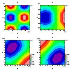
GPhys 1.0.0 における interpolate.rb のテスト部分を掲載します:
require "numru/ggraph"
include NumRu
include NMath
module NumRu
class VArray
def to_g1D
ax = Axis.new().set_pos(self)
grid = Grid.new(ax)
GPhys.new(grid,self)
end
end
end
#< prepare a GPhys object with associated coordinates >
nx = 10
ny = 8
nz = 2
x = (NArray.sfloat(nx).indgen! + 0.5) * (2*PI/nx)
y = NArray.sfloat(ny).indgen! * (2*PI/(ny-1))
z = NArray.sfloat(nz).indgen!
vx = VArray.new( x, {"units"=>"m"}, "x")
vy = VArray.new( y, {"units"=>"m"}, "y")
vz = VArray.new( z, {"units"=>"m"}, "z")
xax = Axis.new().set_pos(vx)
yax = Axis.new().set_pos(vy)
zax = Axis.new().set_pos(vz)
xygrid = Grid.new(xax, yax)
xyzgrid = Grid.new(xax, yax, zax)
sqrt2 = sqrt(2.0)
p = NArray.sfloat(nx,ny)
q = NArray.sfloat(nx,ny)
for j in 0...ny
p[true,j] = NArray.sfloat(nx).indgen!(2*j,1)*sqrt2
q[true,j] = NArray.sfloat(nx).indgen!(2*j,-1)*sqrt2
end
vp = VArray.new( p, {"units"=>"mm"}, "p")
vq = VArray.new( q, {"units"=>"mm"}, "q")
gp = GPhys.new(xygrid, vp)
gq = GPhys.new(xygrid, vq)
r = NArray.sfloat(nz).indgen! * 2
vr = VArray.new( r ).rename("r")
gr = GPhys.new( Grid.new(zax), vr )
d = sin(x.newdim(1,1)) * cos(y.newdim(0,1)) + z.newdim(0,0)
vd = VArray.new( d ).rename("d")
gd = GPhys.new(xyzgrid, vd)
gx = vx.to_g1D
ga = gd + gx
ga.name = "a"
gd.set_assoc_coords([gp,gq,gr,ga])
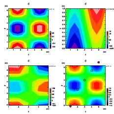
print "GPhys with associated coordinates:\n"
p gd
DCL.swpset('iwidth',700)
DCL.swpset('iheight',700)
DCL.gropn(1)
DCL.glpset("lmiss",true)
DCL.sldiv("y",2,2)
GGraph::set_fig "viewport"=>[0.15,0.85,0.15,0.85]
GGraph::tone gd
GGraph::color_bar
GGraph::tone gd[true,ny/2,true]
GGraph::color_bar
#< prepare coordinates to interpolate >
xi = NArray[1.0, 2.0, 3.0, 4.0, 5.0]
yi = NArray[-0.1, 2.5, 4.0, 5.5, 6.8] # test of extrapolation
vxi = VArray.new( xi, {"units"=>"m"}, "x") # "0.5m" to test unit conversion
vyi = VArray.new( yi, {"units"=>"m"}, "y") # "0.5m" to test unit conversion
pi = NArray.float(6).indgen!*2+10
qi = NArray.float(6).indgen!*2
vpi = VArray.new( pi, {"units"=>"mm"}, "p")
vqi = VArray.new( qi, {"units"=>"mm"}, "q")
ai = NArray[2.0, 4.0]
vai = VArray.new( ai ).rename("a")
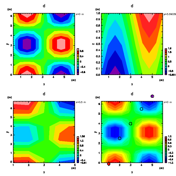
#< test of interpolate >
gxi = vxi.to_g1D
gyi = vyi.to_g1D
gp = GPhys.new(xygrid,vp)
gq = GPhys.new(xygrid,vq)
gi = gd.interpolate(vxi,vyi,{"z"=>0.5})
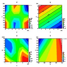
GGraph::tone gi,true,"color_bar"=>true
###gd.interpolate(vxi,vyi,vr,vz) # nust fail by over-determination
gi = gd.interpolate([vxi,vyi])
GGraph::tone gd,true,"min"=>-1.2,"max"=>1.2,"int"=>0.1
GGraph::scatter gxi, gyi, false,"type"=>4,"size"=>0.027,"index"=>3
GGraph::color_scatter gxi, gyi, gi, false,"min"=>-1.2,"max"=>1.2,"int"=>0.1,"type"=>10,"size"=>0.029
GGraph::color_bar
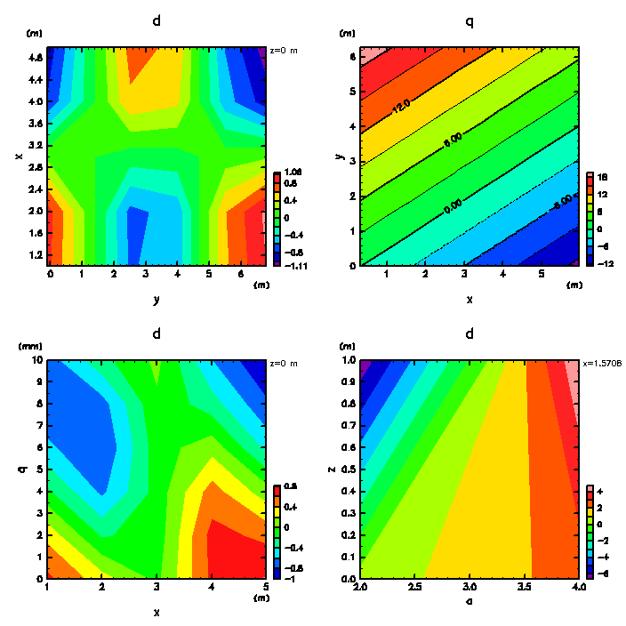
gi = gd.interpolate(vyi,vxi)
GGraph::tone gi,true,"color_bar"=>true
#GGraph::tone gp,true,"color_bar"=>true
GGraph::tone gq,true
GGraph::contour gq,false
GGraph::color_bar
gi = gd.interpolate(vxi,vqi)
GGraph::tone gi,true,"color_bar"=>true
gi = gd.interpolate("y"=>vqi)
gi = gd.interpolate("y"=>vai)
GGraph::tone gi[2,false],true,"color_bar"=>true
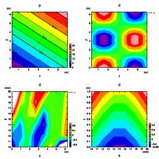
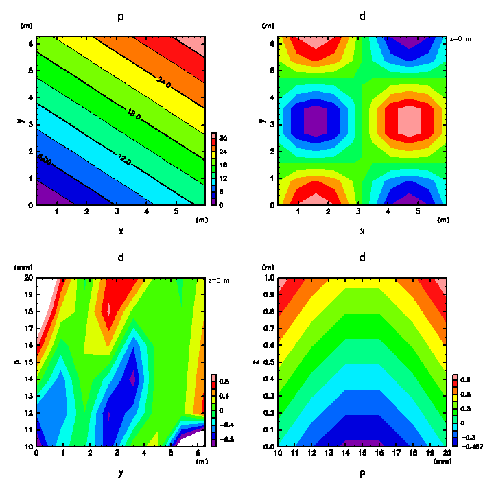
GGraph::tone gp,true
GGraph::contour gp,false
GGraph::color_bar
gi = gd.interpolate("x"=>vpi)
GGraph::tone gd
GGraph::tone gi,true,"color_bar"=>true,"exchange"=>true,"min"=>-1,"max"=>1
gi = gd.interpolate([vpi,vqi])
GGraph::tone gi,true,"color_bar"=>true
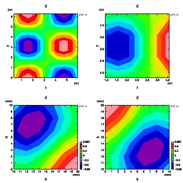
GGraph::tone gd
GGraph::tone gd.cut("p"=>vpi.min.to_f..vpi.max.to_f,"q"=>vqi.min.to_f..vqi.max.to_f),true
gi = gd.interpolate(vpi,vqi)
GGraph::tone gi,true,"color_bar"=>true
gi = gd.interpolate(vqi,vpi)
GGraph::tone gi,true,"color_bar"=>true
gi2 = gd.regrid(gi[false,0])
p "regriding test (should be true):", gi.val == gi2.val
gi = gd.interpolate(vqi,vpi,{"z"=>0.5})
GGraph::tone gi,true,"color_bar"=>true
mask=d.lt(0.7)
missv = -999.0
d[mask.not] = missv
p d[false,0]
dm = NArrayMiss.to_nam(d, mask )
vdm = VArray.new( dm, {"missing_value"=>NArray[missv]}, "d")
gdm = GPhys.new(xyzgrid, vdm)
gi = gdm.interpolate(vpi,vqi)
GGraph::tone gi,true,"color_bar"=>true
#< finish >
DCL.grcls
実行結果
以下にマニュアルを載せます.
interpolate(*coords)Wide-purpose multi-dimensional linear interpolation
This method supports interpolation regarding combinations of 1D and 2D coordinate variables. For instance, suppose self is 4D with coordinates named ["x", "y", "z", "t"] and associated coordinates "sigma"["z"] ("sigma" is 1D and its axis is "z"), "p"["x","y"], "q"["x","y"] ("p" and "q" are 2D having the coordinates "x" and "y"). You can make interpolation by specifying 1D VArrays whose names are among "x", "y", "z", "t", "sigma", "p", "q". You can also use a Hash like {"z" => 1.0} to specify a single point along the "x" coordinate.
If the units of the target coordinate and the current coordinate are different, a converstion was made so that slicing is made correctly, as long as the two units are comvertible; if the units are not convertible, it is just warned.
If you specify only "x", "y", and "t" coordinates for interpolation, the remaining coordinates "z" is simply retained. So the result will be 4 dimensional with coordinates named ["x", "y", "z", "t"], but the lengths of "x", "y", and "t" dimensions are changed according to the specification. Note that the result could be 3-or-smaller dimensional -- see below.
Suppose you have two 1D VArrays, xnew and ynew, having names "x" and "y", respectively, and the lengths of xnew and the ynew are the same. Then, you can give an array of the two, [xnew, ynew], for coord0 as
gp_int = gp_org.interpolate( [xnew, ynew] )
(Here, gp_org represents a GPhys object, and the return value pointed by gp_int is also a GPhys.) In this case, the 1st dimension of the result (gp_int) will be sampled at the points [xnew[0],ynew[0]], [xnew[1],ynew[1]], [xnew[2],ynew[2]], ..., while the 2nd and the third dimensions are "z" and "t" (no interpolation). This way, the rank of the result will be reduced from that of self.
If you instead give xnew to coord0 and ynew to coord1 as
gp_int = gp_org.interpolate( xnew, ynew )
The result will be 4-dimensional with the first coordinate sampled at xnew[0], xnew[1], xnew[2],... and the second coordinate sampled at ynew[0], ynew[1], ynew[2],... You can also cut regarding 2D coordinate variable as
gp_int = gp_org.interpolate( pnew, qnew )
gp_int = gp_org.interpolate( xnew, qnew )
gp_int = gp_org.interpolate( [pnew, qnew] )
gp_int = gp_org.interpolate( [xnew, qnew] )
In any case, the desitination VArrays such as xnew ynew pnew qnew must be one-dimensional.
Note that
gp_int = gp_org.interpolate( qnew )
fails (exception raised), since it is ambiguous. If you tempted to do so, perhaps what you want is covered by the following special form:
As a special form, you can specify a particular dimension like this:
gp_int = gp_org.interpolate( "x"=>pnew )
Here, interpolation along "x" is made, while other axes are retained. This is useful if pnew corresponds to a multi-D coordinate variable where there are two or more corresponding axes (otherwise, this special form is not needed.)
See the test part at the end of this file for more examples.
LIMITATION
Currently associated coordinates expressed by 3D or greater dimensional arrays are not supported.
Computational efficiency of pure two-dimensional coordinate support should be improved by letting C extensions cover deeper and improving the search algorithm for grid (which is usually ordered quasi-regularly).
COVERAGE
Extrapolation is covered for 1D coordinates, but only interpolation is covered for 2D coordinates (which is limited by gt2dlib in DCL -- exception will be raised if you specify a grid point outside the original 2D grid points.).
MATHEMATICAL SPECIFICATION
The multi-dimensional linear interpolation is done by supposing a (hyper-) "rectangular" grid, where each dimension is independently sampled one-dimensionally. In case of interpolation along two dimensional coordinates such as "p" and "q" in the example above, a mapping from a rectangular grid is assumed, and the corresponding points in the rectangular grid is solved inversely (currently by using gt2dlib in DCL).
For 1D and 2D cases, linear interpolations may be expressed as
1D:  zi = (1-a)*z0 + a*z1
2D:  zi = (1-a)*(1-b)*z00 + a*(1-b)*z10 + (1-a)*b*z01 + a*b*z11
This method is extended to arbitrary number of dimensions. Thus, if the number of dimensions to interpolate is S, then 2**S grid points are used for each interpolation (8 points for 3D, 16 points for 4D,...). Thus, the linearity of this interpolation is only along each dimension, not over the whole dimensionality.
USAGE
interpolate(coord0, coord1, ...)
ARGUMENTS
[SPECIAL CASE] You can specfify a one-element Hash as the only argument such as
gphys.interpolate("x"=>varray)
where varray is a coordinate onto which interpolation is made. This is espcially useful if varray is multi-D. If varray's name "p" (name of a 2D coordnate var), for example, you can interpolate only regarding "x" by retaining other axes. If varray is 1-diemnsional, the same thing can be done simply by
gphys.interpolate(varray)
since the corresponding 1D coordinate is found aotomatically.
RETURN VALUE
mouse_cut(dimx, dimy, num=2)Makes a subset interactively by specifying a (poly-)line on the DCL viewport
ARGUMENTS
RETURN VALUE
mouse_cut_repeatregrid(to)Interpolate to conform the grid to a target GPhys object
ARGUMENTS
RETURN VALUE
*1このデータはNOAAのサイトから取得しました.本ファイルには1-2月のデータのみ入ってます.
*2このデータはNOAAのサイトから取得しました.本ファイルには1-2月のデータのみ入ってます.
*3このデータはNOAAのサイトから取得しました.本ファイルには1-2月のデータのみ入ってます.
*4補助座標となる GPhys オブジェクトにおける主座標は,補助座標を与えられる GPhys オブジェクトの主座標の中に含まれてないとなりませんが,theta と uwnd は同じ座標で定義されているので,その条件を満たします


 図b
図b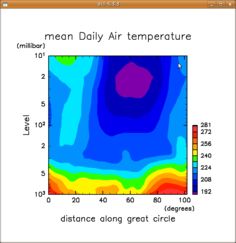
 図
図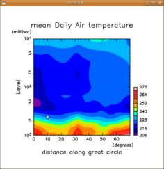