Held and Suarez (1994) dynamcal core experiment
A method to perform dynamical core experiment proposed by Held and Suarez (1994) is described.
Following physical processes are used in this experiment.
- Newtonian relaxation of the temperature field to a zonally symmetric state
- Rayleigh damping of low-level winds
- processes related to moisture are excluded.
- Dry convective adjustment
Overview
This experiment does not require additional data, such as SST data. So, the experiment is performed with the following 3 steps:
- Compliation of main program etc.
- Preparation of a directory for experiments
- Makeing initial data
- Execution of experiments
Compliation of main program etc.
Move to the HS94 experimental directory and compile main program etc. to generate the executable files.
$ cd execsrc/hs94                        (Move to HS94 directory)
$ make all                               (Compie execution files)
Preparation of a directory for experiments
Running the executable will generate a large number of NetCDF files, so we recommend creating a directory for your experiments and placing your input and output files there. For example, to set up ./exp as your experiment directory, executre the following command to copy the configuration files for initial value generation and for the experiment.
$ mkdir exp ; cd exp
$ cp ../exp_setup_files/init_data_hs94_T21L20.conf .
$ cp ../exp_setup_files/dcpam_hs94_T21L20_short.conf .
Makeing initial data
Use `dcpam_init_data_hs94` and `init_data_hs94_T21L20.conf` to create the initialization file `init_T21L20.nc`.
$ ../dcpam_init_data_hs94 -N=init_data_hs94_T21L20.conf
                      :
*** MESSAGE [restart_file_io] ***  ----- Initialization Messages -----
*** MESSAGE [restart_file_io] ***  Input::
*** MESSAGE [restart_file_io] ***    InputFile  = <Non>
*** MESSAGE [restart_file_io] ***    ** Initial data is generated in "initial_data" module
*** MESSAGE [restart_file_io] ***  Output::
*** MESSAGE [restart_file_io] ***    OutputFile = init_T21L20.nc
*** MESSAGE [restart_file_io] ***    IntTime    = 365. [day]
*** MESSAGE [restart_file_io] ***  -- version = $Name:  $$Id: restart_file_io.f90,v 1.26 2025/09/17 22:00:00 takepiro Exp $
*** MESSAGE [HistoryCreate1] ***  "init_T21L20.nc" is created (origin=0. [sec])
*** MESSAGE [HistoryClose] ***  "init_T21L20.nc" is closed
Execution of experiments
Using the NAMELIST file dcpam_hs94_T21L20.conf, run dcpam_main_hs94 as follows.
$ ../dcpam_main_hs94 -N=dcpam_hs94_T21L20_short.conf

*** MESSAGE [dcpam_main] ***  Run: Held and Suarez (1994) benchmark test
                  :
*** MESSAGE [timeset] ***  ----- Initialization Messages -----
*** MESSAGE [timeset] ***    StartTime  = 0. [day]
*** MESSAGE [timeset] ***    EndTime    = 10. [day]
*** MESSAGE [timeset] ***    DelTime    = 30. [min]
*** MESSAGE [timeset] ***               = 1800. [sec]
                  :
                  :
*** MESSAGE [fileset] ***  ----- Initialization Messages -----
*** MESSAGE [fileset] ***    FileTitle       = Held and Suarez (1994) benchmark test
*** MESSAGE [fileset] ***    FileSource      = dcpam5 (http://www.gfd-dennou.org/library/dcpam)
*** MESSAGE [fileset] ***    FileInstitution = GFD Dennou Club (http://www.gfd-dennou.org)
*** MESSAGE [fileset] ***  -- version = ....
*** MESSAGE [gridset] ***  ----- Initialization Messages -----
*** MESSAGE [gridset] ***    nmax = 21
*** MESSAGE [gridset] ***    imax = 64
*** MESSAGE [gridset] ***    jmax = 32
*** MESSAGE [gridset] ***    kmax = 20
*** MESSAGE [gridset] ***  -- version = ....
                  :

########## PREDICTION OF CALCULATION ###########
Start Date             2009-03-06T08:26:41+09:00
Current Date           2009-03-06T08:26:45+09:00
Progress     20.00%  [*****                    ]
Remaining CPU TIME      0.160000E+02
Completion Date        2009-03-06T08:27:01+09:00

                  :

############## CPU TIME SUMMARY ################
held_suarez_1994       0.165611E+01
dynamics_hspl_vas83    0.191452E+02
timefilter_asselin19   0.264027E+00
others                 0.896038E+00
------------------------------------------------
       TOTAL TIME =    0.219614E+02
In this case, a time integration over 10 days is performed. The spatial resolution is T21L20 (64 longitude grid points, 32 latitude points, and 20 vertical layers). The calculation results are output as U.nc and Temp.nc. In addition, the restart file is output as rst.nc.
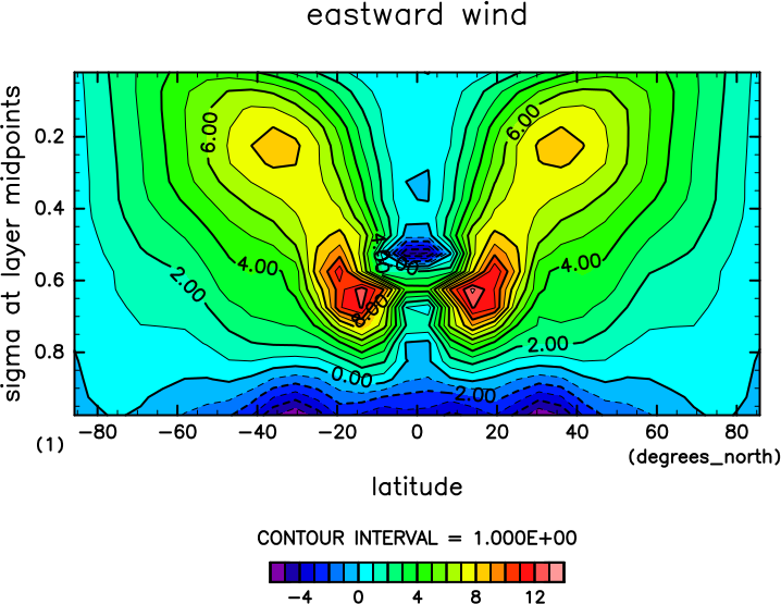
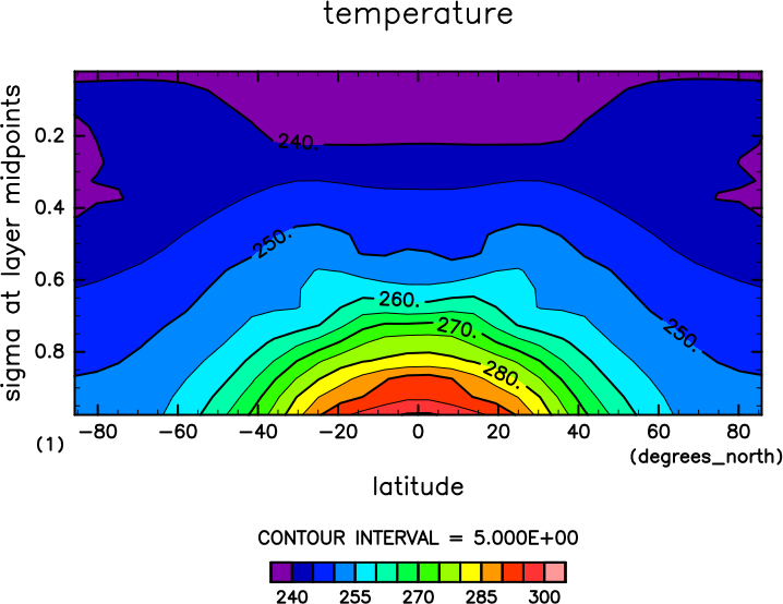
The zonal averaged longitudinal wind and temperature distributions at 10 days later are shown in the figures below. These figures were created using the `gpview` command, which is included in the GPhys package, as shown below.
$ gpview U.nc@U,time=10 --mean lon --int 1 --noannotate
$ gpview Temp.nc@Temp,time=10 --mean lon --int 5 --noannotate
For more detailed information on analysis and visualization, please refer to here.
Saving data
If you would like to keep the results of the numerical experiment, please create a sub directory ("data01" for example), move the files, and keep the current directory neatly.
$ mkdir data01
$ mv *.conf *.nc *.log data01/
You can output the results of the numerical experimet concurrently with the execution. Please refer to "Change output settings" in Change experimental setup and try to configure "FilePrefix" variable in NAMELIST ">ool_historyauto_nml".
MPI Parallel Computing: For More Advanced Experiments
Let's try performing a longer-duration integration using MPI 4 parallel computing. First, save the data calculated so far to a separate directory, then copy the configuration file for the long-duration integration (1,000 days).
$ cp ../exp_setup_files/dcpam_hs94_T21L20.conf .
Create the initial values for parallel processing. The executable files whose names end with _mpi are for MPI parallel computing.
$ mpirun -n 4 ../dcpam_init_data_hs94_mpi -N=init_data_hs94_T21L20.conf
`mpirun` is the command for running parallel computations, and `-n 4` is the option that specifies a 4-way parallel computation. Please adjust these commands and options according to the compiler and system you are using. Unlike in the case of a single-CPU calculation, four initial data files—from `init_T21L20_rank000000.nc` to `init_T21L20_rank000003.nc`—will be created.
We will perform a long-duration integration. Since this will take some time, we will redirect the output to dcpam_hs94_T21L20.log.
$ mpirun -n 4 ../dcpam_main_hs94_mpi -N=dcpam_hs94_T21L20.conf >& dcpam_hs94_T21L20.log &
$ tail -f dcpam_hs94_T21L20.log
The `tail` command is a convenient way to monitor the progress of the calculation. To exit the `tail` command, press Ctrl-C.
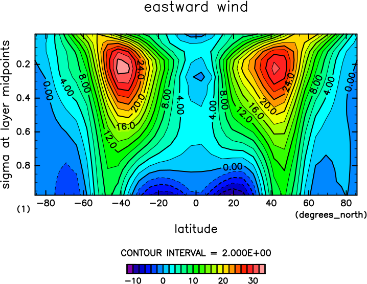
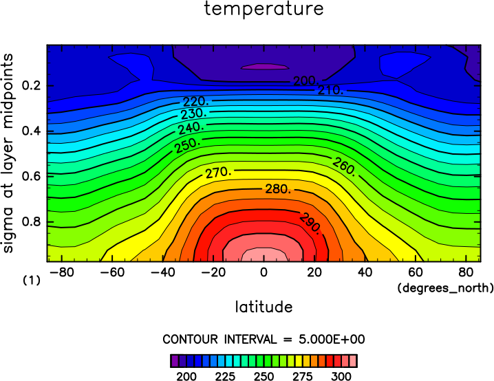
The output for each variable is also split into four files, ranging from *_rank000000.nc to *_rank000003.nc. The figure below shows the results after 1,000 days, plotted using gpview. By specifying the file path as *_rank00000\*.nc, you can load and merge the split files.
$ gpview U_rank00000\*.nc@U,time=1000 --mean lon --int 2 --noannotate
$ gpview Temp_rank00000\*.nc@Temp,time=1000 --mean lon --int 5 --noannotate
In Held and Suarez (1994), the spatial resolution is equivalent to T63L20 (192 longitude grid points, 96 latitude grid points, and 20 vertical layers), and the data were time-integrated over 1,200 days.